<
!— WordPress Article: Understanding the IF formula in Excel with practical examples —>
The IF function in Excel is one of the most used to make automatic decisions in your tables: predicting if a grade is sufficient, categorizing sales, generating conditional messages… Yet, sometimes we feel a bit lost between syntax, logical values, and nested formulas. In this article, I guide you step by step, with practical cases I have experimented with on real workbooks, so that you can quickly gain efficiency.
What is the IF function?
In a few words, IF tests a condition then returns a result if the condition is true, and another if it is false. It is a simple way to automate choices in Excel, rather than going through manual filters or repetitive sorts.
Detailed syntax of IF
Function arguments
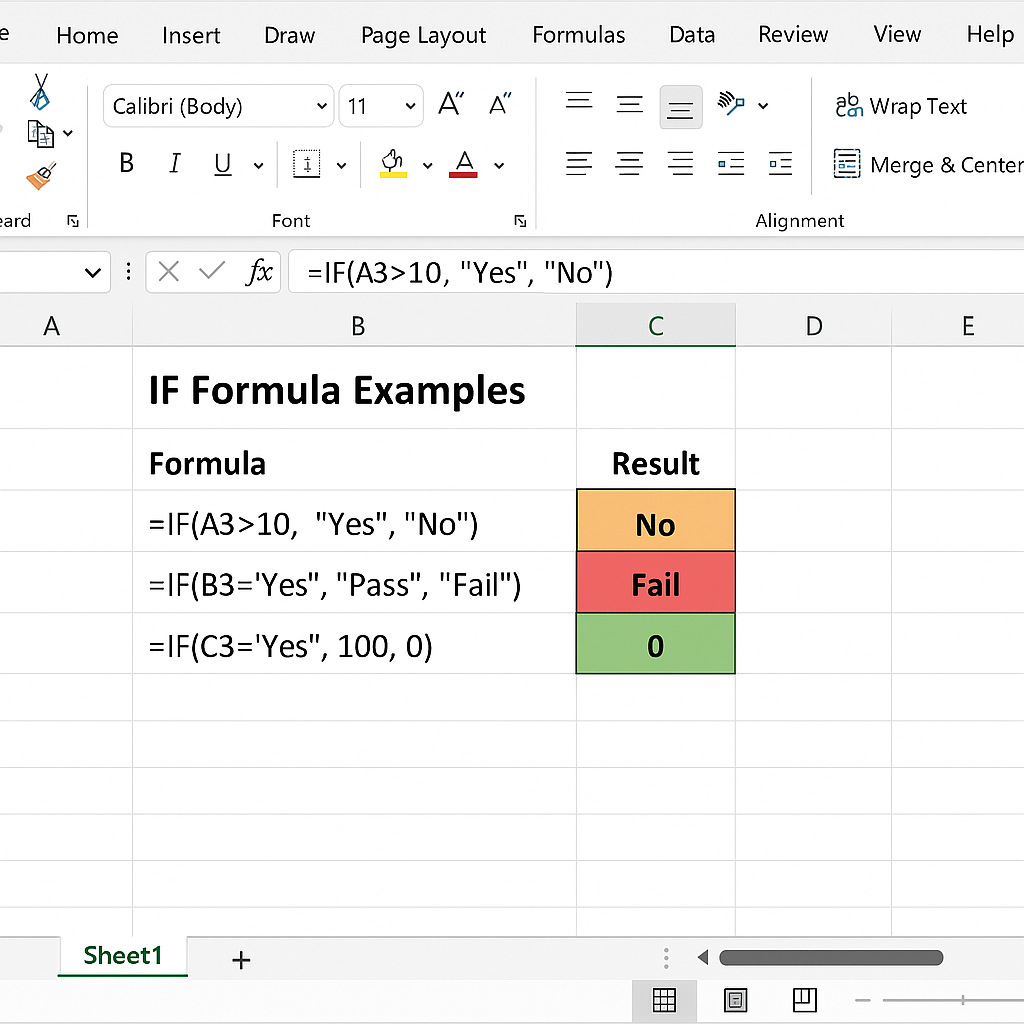
- logical_test: the expression you want to evaluate (e.g., A2>10).
- value_if_true: what Excel returns when the test is true (text, number, formula…).
- value_if_false: what Excel returns if the test is false.
Concretely, the formula is written as follows: =SI(test_logique, valeur_si_vrai, valeur_si_faux). Nothing simpler, but it is in the combinations that the trouble lies.
Practical examples
1. Numeric test: evaluating a grade
Imagine a table of school results; you want to display “Passed” if the grade is ≥ 50, “Failed” otherwise. You use:
=SI(B2>=50, "Admis", "Ajourné")
Here B2 contains the grade. With each copy downwards, Excel compares the value and automatically displays the textual response.
2. Textual test: converting Yes/No to binary
In a survey file, it happens that the answers “Yes” and “No” are written out in full. For statistical analysis, you can transform “Yes” into 1 and “No” into 0:
=SI(C2="Oui", 1, 0)
This conversion is useful before applying sums or averages, because Excel does not calculate directly on text.
3. Nested IFs: classifying according to multiple levels
If you want to assign a mention according to the grade, you must test several ranges:
| Grade | Mentions |
|---|---|
| >= 85 | “Very Good” |
| >= 70 and < 85 | “Good” |
| >= 50 and < 70 | “Sufficient” |
| < 50 | “Insufficient” |
The most classic way is to chain three IFs:
=SI(D2>=85, "Très Bien", SI(D2>=70, "Bien", SI(D2>=50, "Suffisant", "Insuffisant")))
If you find this formula a bit long, know that Excel 2016+ offers IFS to simplify writing multiple tests.
Combining IF with Other Functions
To take automation even further, IF is combined with other functions: AND or OR to cross multiple criteria, CONCATENATE to create dynamic messages, or the VLOOKUP function to cross two tables based on a condition.
- IF+AND:
=SI(ET(A2>=60; B2>=60); "Admis"; "À revoir"). - IF+OR:
=SI(OU(C2>"France"; C2="Belgique"); "UE"; "Hors UE"). - IF+CONCATENATE:
=SI(E2>100; CONCATENER("Attention : ";E2); "OK").
Best Practices and Pitfalls to Avoid
- Check the consistency of types: text, number, or date must match your test.
- Favor a clear order when nesting multiple IFs to avoid priority errors.
- Remember that Excel allows up to 64 levels of nested IFs; beyond that, the formula becomes unreadable.
- If you have too many conditions, try the IFS function (available since Excel 2016).
- For fast calculations on large tables, limit the number of volatile formulas (IF is not volatile, but its partners can be).
Conclusion
The IF function is a cornerstone of conditional analysis in Excel: it allows you to convert numbers into keywords, trigger automated alerts, and structure dynamic reports without coding. With a bit of practice and some tips (IFS, AND, OR), you will move from basic use to a true homemade business intelligence tool.
Practice on real cases to gain confidence, and remember to combine IF with other advanced functions as soon as your needs expand.


