| Key Points | Details to Remember |
|---|---|
| 🔍 Definition | Search for a value in the first column of a table |
| ⚙️ Syntax | =VLOOKUP(value; table; index; [sorted]) |
| 📌 Parameters | value, table_array, col_index_num, range_lookup |
| ✅ Exact or Approximate | FALSE for exact, TRUE for approximate |
| 🔄 Advanced Uses | Combinations with INDEX/MATCH or dynamic data structures |
| 💡 Best Practices | Lock ranges, name your tables, handle errors |
One April morning, my colleague Julie said to me: “Do you really know VLOOKUP? Because right now, I’m struggling to merge two lists!” I saw her screen filled with #N/A and empty cells… Without knowing it, she had just awakened my passion for Excel formulas. Since then, I’ve been sharing tips to master this function and I’m telling you all about it here.
Understanding the VLOOKUP Function
VLOOKUP, or RECHERCHEV in the French version of Excel, is used to fetch information from a table based on a reference value. It’s super handy when working with product lists, customer databases, or even inventories. The function looks for the “key” you specify in the first column of the table and returns content located in the same row.
Syntax and Parameters
Here is the basic structure:
=VLOOKUP(lookup_value; table_array; col_index_num; [range_lookup])
- lookup_value: the data you want to find (a reference, a name…)
- table_array: the range of cells where Excel will search
- col_index_num: the column number within the range that contains the value to return
- range_lookup: specify FALSE for an exact match, TRUE (or omitted) for an approximate match
Simple Example
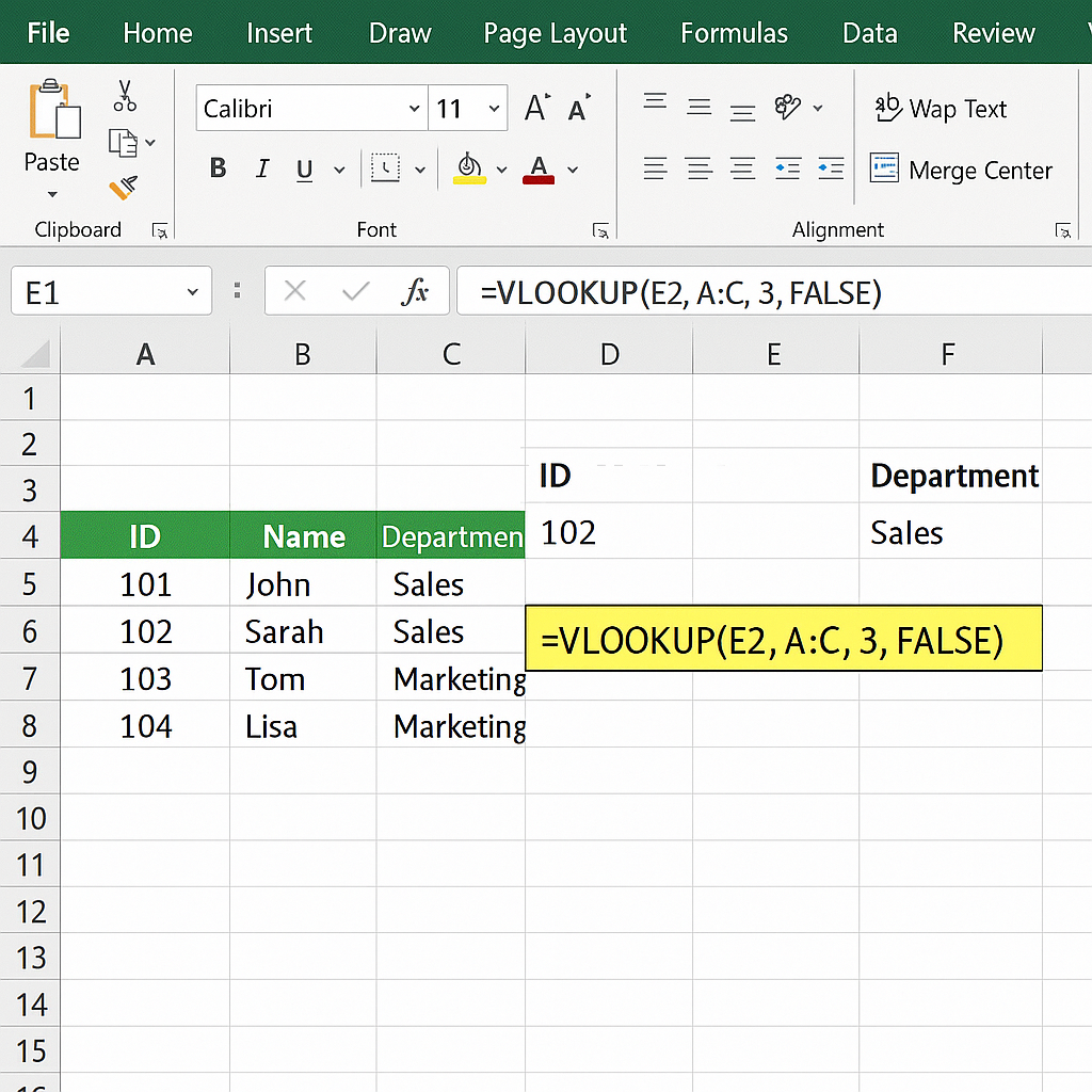
Imagine a “Products” file with product codes in column A and their prices in column B. You want to display the price corresponding to the code entered in D2:
=VLOOKUP(D2; A2:B100; 2; FALSE)
Here, Excel will look for the value in D2 within A2:A100. When it finds it, it returns the corresponding cell from column B.
Parameter [range_lookup]: exact or approximate
Exact vs Approximate Lookup
The fourth argument is often a source of errors.
• FALSE → precise search: returns #N/A if the value is not strictly identical.
• TRUE (or empty) → approximate search: the first column must be sorted in ascending order, otherwise results will be random.
Tip: if you forget to sort, you risk significant discrepancies, especially on date or price ranges.
Best Practices to Avoid Errors
- Lock your table_array cells with the $ sign (e.g., A$2:B$100).
- Name ranges via the Formulas tab > Name Manager for better clarity.
- Handle errors with IFNA or IFERROR to display a friendly message.
Advanced Uses
Once the basics are mastered, you can combine VLOOKUP with other tools to gain flexibility:
Combine with INDEX and MATCH
INDEX/MATCH offers more power on the “left” columns and avoids the limitation of VLOOKUP which can only look to the right.
Typical formula: =INDEX(B2:B100, MATCH(value, A2:A100, 0)).
It is often a more robust duo, especially if your database evolves or you add columns.
Troubleshooting: handling common errors
- #N/A: the value was not found → check spelling, case, and absence of invisible spaces.
- #REF!: no_index_col out of range → adjust the column number.
- Incorrect results: table not sorted in approximate mode → switch to FALSE or sort correctly.
Tips to optimize your searches
You can go further:
- Use HLOOKUP for the same logic on horizontal rows.
- Deploy XLOOKUP (Excel 365) for more flexible and dynamic searches.
- Apply conditional formatting to highlight searched values.
- Save your formulas as macros or use Power Query to automate massive updates.
FAQ
-
What distinguishes VLOOKUP from XLOOKUP?
XLOOKUP is more recent: it handles searches in both directions, returns a default value if nothing is found, and simplifies the syntax.
-
Why does my formula always return the same value?
Check that your table_array is not fixed on a single row, and that no_index_col has not been inadvertently set to 1.
-
How to search for multiple criteria?
Create a combined key (e.g. =A2&B2) in a column, then search for this new value with VLOOKUP.


